sampling from an arbitrary distribution
The first thing you probably found
If you ask a random person (conditioned on them being a reasonable target for this question) how to sample from an arbitrary distribution, you are pretty likely to get this answer: “Just sample form a uniform distribution between 0 and 1, and invert the samples using the inverse cdf”. This is a wonderfully elegant solution, and we might as well start by looking at how it works. We’ll use a really simple PDF for lillustrative purposes: \(\text{pdf}(x) = 2x\), which will be normalized with a domain of \(x \in [0,1]\).
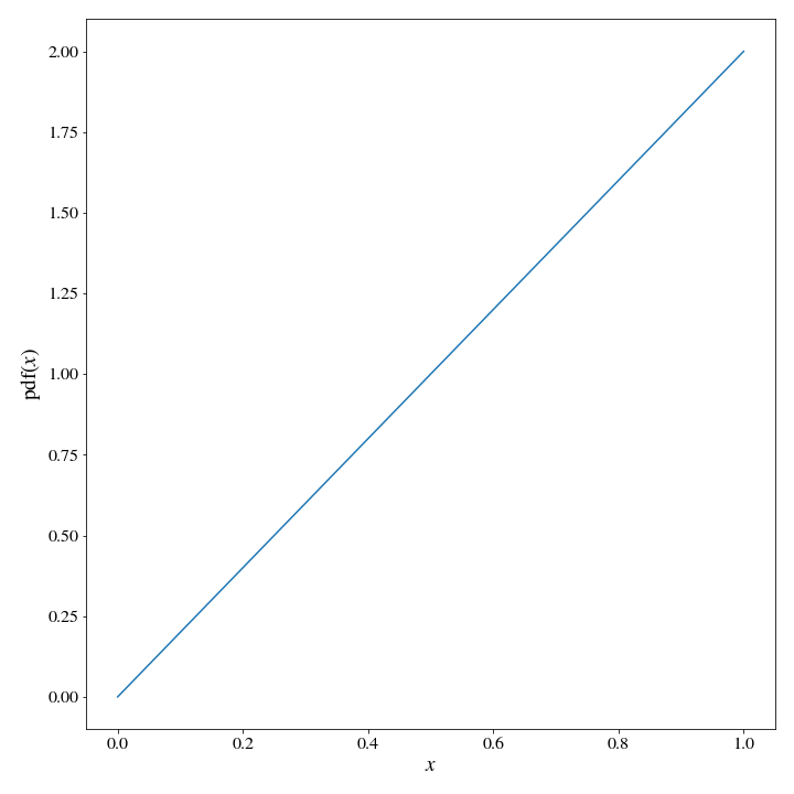
We can calculate the cdf readily: \(\text{cdf}(x)= x^2\), so the inverse cdf is a square root. With this information, it is trvial to sample say, 1,000,000 samples from the initial pdf:
# sample 1,000,000 values from cdf(x)
cdf_samples = np.random.uniform(0,1, 1_000_000)
# invert them, by taking the square root
x_vals = np.sqrt(cdf_samples)
We can plot a histogram of the x_vals to see if it worked:
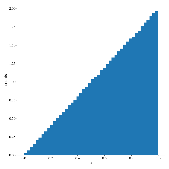
It did.
The catch
You did need to invert the cdf, which can be a bit of a bummer. Or course, since you are working on a computer (probably) you can probably do a pretty good job of numerically integrating the pdf and building up a numeric inverse instead. But the real issue with this method is how it scales into higher dimensions.
Unfortunately for anyone who lives or thinks in more than 1Dimension: the inverse cdf is only guarateed to exist and/or be well defined in a single dimension. Multivariate distributions typically have multi-valued inverse cdf relations. Just imagine a symmetric 2 dimensional gaussian distribution. There will be a circle of coordiantes at a radius \(r\) from the peak of the gaussian that all share the same probability, so just choosing a probability between \(0\) and \(1\) will not give you an unambiguous point in coordinate space. Additionally, the size of these regions depends on how far from the center you are– so it doesn’t evem make sense to sample the probability uniformly anyway. So, let’s work on a method that will work for multivariate distributions.
First pass at a new method
Here is the idea:
- we generate a point \(Y\) in our domain using a uniform distribution
- we calcualte the probability \(\text{pdf}(Y)\) of that point using the known target pdf
- we genenrate a random uniform variable \(U \in [0,1]\),
- we accept the point Y as being part of our sample if \(U \leq \text{pdf}(Y)\) The idea behind this is intuitive. We are more likely to accept the higher probability events and less likely to accept the low probability ones, and the ratio between these acceptances is the ratio of ther relative probabilities. Thus, we would expect our list of accepted \(Y\) values to follow the target pdf. Sure, we have lost some efficiency, because we have to spend resources making samples that will be rejected– but that is the tradeoff ofr this more general method. Let’s take a look at how this works in practice, using the same target distribution as above:
def target_dist(x):
    return 2*x

Y = np.random.uniform(0,1,N)
prob_fY = target_dist(Y)
U = np.random.uniform(0,1,N)
accepted_samples = Y[U <= accept_probs]
And the histogram of accepted samples, to see if it worked…
It did not.
Rejection Sampling
Well, what happened was that \(\text{pdf}(x)\) was actually larger than 1 for half of the values– so we were unable to reject those samples. The problem has to be scaled properly for this to work. We made the classic mistake of thinking of the pdf as giving the probabilities of each point in the space when it actually only gives us density. The solution here is to talk about ratios of pdf’s instead. This intuitive method we have been trying out is sometimes called ‘rejection sampling’, and is one of many monte-carlo algorithms that solve difficult problems generating a variable from a simple case and the accepting or rejecting is based on the more complicated problem. A corrected version of the method goes like this:
- we want to generate a realization of the random variable \(X\) distributed according to a “target distribution” \(f(x)\)
- we generate a random variable \(Y\) using an easy to sample from “proposal distribution” \(g(Y)\)
- we genenrate a random uniform variable \(U \in [0,1]\),
- we accept the point Y as being part of our sample if \(U \leq \frac{f(Y)}{M\cdot g(Y)}\)
- M is a constant parameter, chosen so that the ratio on the RHS of the inequality never surpasses 1
Assuming that both distibutions are normalized, we can use \(M\) as a measure of the efficiency of the algorithm because \(1/M\) is approximately the probability of accepting a sample \(Y\). Revisiting our previous case, we can see that with the uniform distribution having \(g(Y)=1\) in our domain that we will need \(M=2\) to ensure the ratio of \(\frac{f(Y)}{M\cdot g(Y)} \leq 1\) for our entire domain. And, we expect to throw out \(\sim 50\%\) of our geenrated \(Y\) values. So we expect to generate \(2N\) samples of \(Y\) to generate \(N\) samples of \(X\). Let’s make a little function to do the rejection sampling for us
Now, to try it out. We run the exact same code as before. Except, we add in the effect of \(M\):
Y = np.random.uniform(0,1,N)
prob_fY = target_dist(Y)
U = np.random.uniform(0,1,N)
# add in M
M=2
accepted_samples = Y[U <= accept_probs/M]

#do quick histogram to verify
fig, ax = plt.subplots()
ax.hist(accepted_samples, bins=50, density=True);
ax.set_ylabel('counts');
ax.set_xlabel('$x$');
ax.set_title(f'generated {n} samples, accepted {len(accepted_samples)}')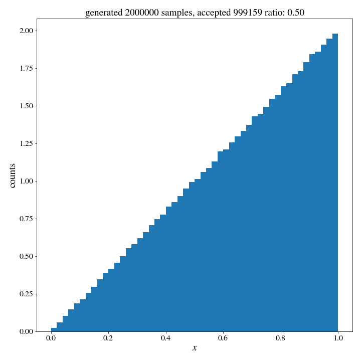
And there we go! This is rejection sampling in a nutshell. Of course, it’s probably clear as this point that a uniform distribution is not the most efficient distribution for our target pdf. Ideally, we want the proposal distribution to be as close to the target distribution as we can make it, while still being easy to sample from. Could we leverage the ability to easily sample from gaussians to do a better job? At first glance it seems like a bad idea: the Gaussian is totally symmetric and our target_dist is absolutely not. However, by generating a normally distributed variable \(G\) and taking the absolute value, we can create a one sided distribution that is well suited for our purposes.
With \(Y = 1-\text{abs}(G(0,\sigma))\), we can see that the distribution of \(Y\) looks quite similar to our target distrbution, with a value of \(M\) that is quite close to \(1\)
from scipy.stats import norm

class one_sided_norm():
    def __init__(self, x0, sigma):
        self.norm = norm(loc=x0, scale=sigma)

    # we have to redefine the pdf here because taking the absolute value
    # effectively halves the domain and doubles the density
    def one_sided_pdf(self,x):
        return 2*self.norm.pdf(x)

fig, ax = plt.subplots()
xt= np.linspace(-1,1)
x= np.linspace(0,1)

ax.plot(x, target_dist(x), label='target_pdf')

#choose some values by guess and check until it looks right
sigma = .45
M =1.2

proposal_dist = one_sided_norm(0, sigma)

ax.plot(1-np.abs(xt), M * proposal_dist.one_sided_pdf(xt), label='$M\cdot $transformed gaussian')
ax.set_xlim(0,1)
ax.set_ylabel('pdf$(x)$');
ax.set_xlabel('$x$');
fig.legend()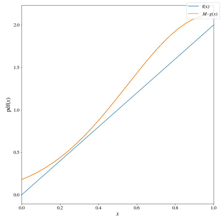
We can see that the ratio \(\frac{f(Y)}{M\cdot g(Y)}\) will always be less than one, guaranteeing a good sample of our target distribution; but, at the same time, it will often be very close to one guaranteeing a high degree of efficiency with accepting our genenrated samples.
Now that we have the hang of it, lets make a time saving function to do this rejection sampling for us:
def rejection_sample(N, target_pdf, proposal_dist, m):
    # N is the number of samples we generate from the sampling dist
    # target_pdf is a function that return the probability density at its argument as an array
    # proposal_dist is an object with a method .sample(k) that returns an array of k samples and their probability density
    # m is the scaling parameter discussed above

    y, prob_gy = proposal_dist.sample(N)
    accepted_samples = y[np.random.uniform(0,1,N) < target_pdf(y)/(m*prob_gy)]

    # here we return both the accepted sample array, and also the ratio to verify if 1/M is truly the prob of acceptance
    return accepted_samples, len(accepted_samples)/N

# redefine our one_sided_norm class to have the method we need for the rejection_sample function
class one_sided_norm():
    def __init__(self, x0, sigma):
        self.norm = norm(loc=x0, scale=sigma)

    # we have to redefine the pdf here because taking the absolute value
    # effectively halves the domain and doubles the density
    def one_sided_pdf(self,x):
        return 2*self.norm.pdf(x)

    def sample(self, N):
        G = self.norm.rvs(N)
        return 1-np.abs(G), self.one_sided_pdf(G)
With these definitions, rejection sampling is as simple as running the following few lines:
M=1.2
sigma= .45
# define the proposal distribution
proposal_dist = one_sided_norm(0, sigma)
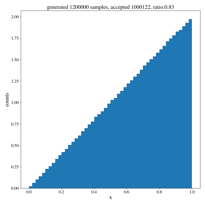
accepted_samples, ratio = rejection_sample(int(N*M), target_dist, proposal_dist, M)Now, with the obligatory histogram of accepted samples to see how we did…
Next steps
Ok, so we got better sample efficiency by handcrafting a gaussian to fit our pdf, but that kind of fine tuning by hand isnt really a scaleable option. Additionally, the extra efficiency needs to offset the extra computational time it takes to sample from the gaussian rather than the uniform distibution. In the next installment we will go over some attempts to automate the process of creating a proposal distribution and also about the pros and cons of using un-normalized distributions.