return of the "sampling from an arbitrary distribution"
note: part 2 of a series on sampling from arbitrary distrbutions, I suggest reading the first one before continuing
Refresher
At the end of the last insallment, we have settled on using a rejection sampling method to generate samples from a random variable \(X\) with a known, but completely arbitrary distribution functions \(f(x)\). A quick review of the method is the following:
- we generate a random variable \(Y\) using an easy to sample from “proposal distribution” \(g(Y)\)
- we generate a random uniform variable \(U \in [0,1]\),
- we accept the point \(Y\) as being part of our sample if \(U \leq \frac{f(Y)}{M\cdot g(Y)}\)
- the accepted \(Y\) values will be distributed the same as \(X\) is
M is a constant parameter that we need to set to ensure the ratio of \(\frac{f(Y)}{M\cdot g(Y)} \leq 1\) for our entire domain. Assuming that both distibutions are normalized, this method works best when \(M\) is as close to \(1\) as possible. There are, of course, other factors to consider– such as the efficiency of your sampling algorithm for \(Y\).
We left off thinking about ways to generate the proposal distribution \(g(x)\) and find the value of \(M\) automatically.
Using np.histogram
One method to accomplish this, is to make a histogram. A normalized histogram is nothing more than a piecewise linear pdf. This is the logical extension of using a uniform distribution as the proposal distribution. Let’s make a Histogram distibution object that holds bins and counts, with the ability to give us the pdf and sample from itself:
class HistDist:
    def __init__(self, counts, bins):
        self.counts = counts
        self.bins = bins
        self.histogram = self.counts, self.bins

    def pdf(self, x):
        def square_step(x, lims, height):
            return height*(np.heaviside(x-lims[0],0) + np.heaviside(lims[1]-x,1)-1)
        return sum( [ square_step(x, self.bins[i:i+2], self.counts[i]) for i in range(len(self.bins)) ] )
    def sample(self, N):
        indices = np.random.choice( range(len(self.counts)), size=N, p=self.counts/self.counts.sum())
        Y = np.random.uniform(self.bins[indices],self.binsb[indices+1])
        prob_Y = self.counts[indices]
        return Y, prob_Y
We should also bring back our old target distribution:
def target_dist(x):
    np.asarray(x)[np.asarray(x)<0]=0
    np.asarray(x)[np.asarray(x)>1]=0
    return 2*x
Ok, let’s see how this works in practice
x = np.linspace(0,1,100)
# make a normalized numpy histogram with 5 bins, weighted by the known distribution weights
proposal_dist = HistDist(*np.histogram(x, weights=target_dist(x), bins=5, density=True))
# well plot both the target and proposal disributions, for a reality check
fig, ax = plt.subplots()
ax.stairs(*proposal_dist.histogram)
ax.plot(x, target_dist(x))
ax.set_ylabel('pdf$(x)$');
ax.set_xlabel('$x$');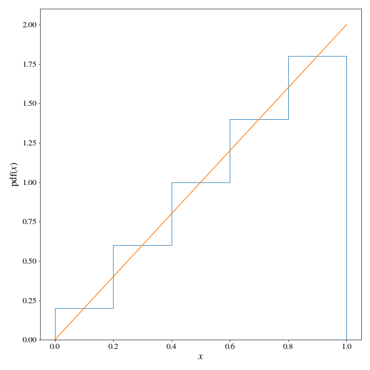
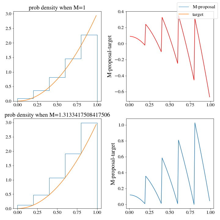
We can see pretty clearly that the target distribution density is significantly lower than that of the proposal distribution as several points, so we will need to find a appropriate value for \(M\). Let’s write some code to do this for us, since we are moving in the direction of automating this whole process:
def find_M(target, proposal, x, M_start=1, plot=True):
    # just ignore the endpoints since the probabiity can go to zero
    x = x[1:-1]
    diff = proposal.pdf(x) - target(x)
    diff_min, x_min = diff[np.argmin(diff)], x[np.argmin(diff)]

    if plot:
        fig, ax = plt.subplots(2,2,figsize=(10,10))

        ax[0,0].stairs(*proposal.histogram, label='M$\cdot$proposal')
        ax[0,0].plot(x, target(x), label='target')
        ax[0,0].set_title(f'prob density when M=1')
        ax[0,1].set_ylabel('M$\cdot$proposal-target')
        ax[0,1].plot(x, diff, c='r')
        fig.legend()

    M = M_start
    # everything else above is for plotting purposes, here is the actual M minimizing
    # we want the smallest difference between M*proposal(x) and target(x) to be positive, and small
    while not np.isclose(diff_min, 0, atol=.001, rtol=.001) or diff_min < 0:
        M = target(x_min)/proposal.pdf(x_min)
        diff = M*proposal.pdf(x)-target(x)
        diff_min, x_min = diff[np.argmin(diff)], x[np.argmin(diff)]
        print(f'M={M}, dff_min:{diff_min}')

    if plot:
        ax[1,1].plot(x, diff)
        ax[1,0].stairs(M*proposal.histogram[0], proposal.histogram[1])
        ax[1,0].set_title(f'prob density when M={M}')
        ax[1,0].plot(x, target(x))
        ax[1,1].set_ylabel('M$\cdot$proposal-target')

    return(M, diff_min)
To generate N samples, we run the following
M, _ = find_M(target_dist, proposal_dist, x)
n = int(N*M)
accepted_samples, ratio = rejection_sample(n, target_dist, proposal_dist, m=M)
Here is the plot we get out from the \(M\) minimization
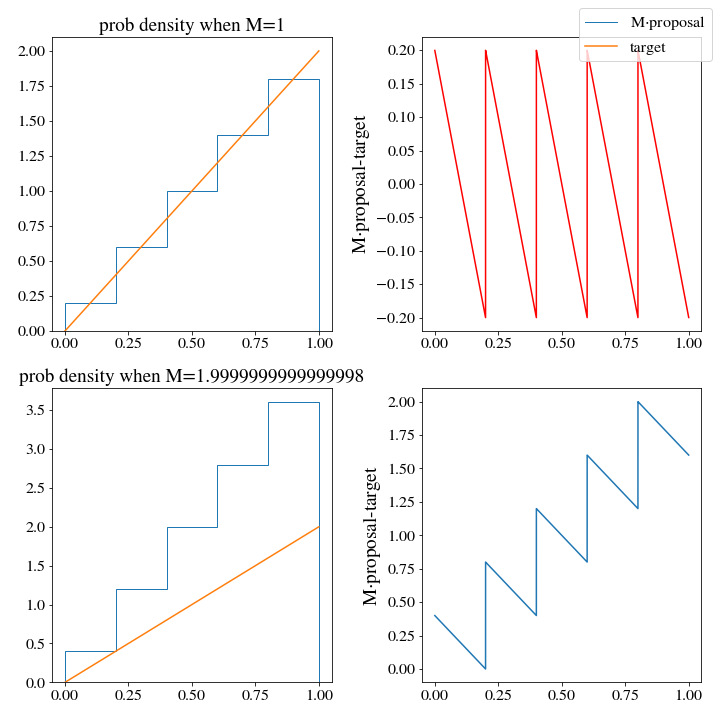
Interestingly, the optimal \(M\) turns out to be the same as we had for the uniform distribution. The problem will not be solved by more bins either, or a finer mesh along \(x\) when training M. We would still have to generate 2 samples on average to get 1. We need a better histogram, one that doesn’t generate densities that are so wildly above the target pdf.
Making our own histogram
Since we can’t rely on the built in numpy histogram function, we will simply build it ourselves. The fact is that while a weighted histogram did achieve what we wanted, it was really totally overkill. We can actually evaluate the target pdf at any point in the domain, so there is no reason to use more than \(m+1\) points for a \(m\) bin histogram. We can set the height of each bin by hand to be the maximum between the left and right endpoints.
def upper_hist(bins, target_dist, density=False):
    # calculate the value of the pdf at both ends of each bin, and set the bins weight to be the maximum between them.
    counts = np.max( (target_dist(bins[:-1]),target_dist(bins[1:])), axis=0 )
    # normalize the counts
    if density:
        norm = sum(np.diff(bins)*counts)
        counts = counts/norm
    return counts, bins
Let’s also use a quadratic pdf this time; which would work even more poorly using the naive histogram approach we used above:
def target_dist(x):
    np.asarray(x)[np.asarray(x)<0]=0
    np.asarray(x)[np.asarray(x)>1]=0
    return 3*x**2
We’ll compare both methods, by making two different proposal distributions:
hist_x = np.linspace(0,1,100)
old_proposal = HistDist(*np.histogram(hist_x, weights=target_dist(hist_x), bins=5, density=True))

bins = np.linspace(0,1,6)
proposal = Hist_Dist(*upper_histogram(bins, target_dist, density=True))
If we plot both histograms, there seems to only be a little difference between the two:
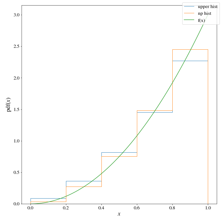 However, there are huge consequences when it comes to the efficiency of these two histogram distributions. WHen we use the np histogram method, \(M\approx 3\):
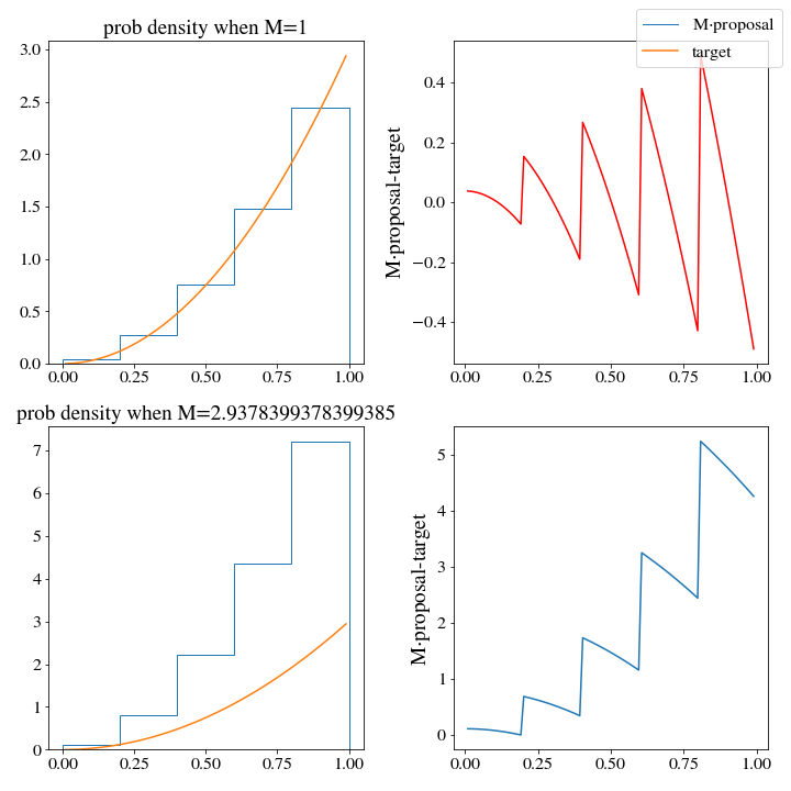 While \(M\approx1.3\) for the upper histogram!
 This means that we should expect the upper histogram to be more than twice as efficient at generating samples of the target distribution (and this will be borne out if you test it as well, go ahead and give it a try.)
Unnormalized distributions
You may have already intuited that this will work for unnormalized distributions too. If the distributions \(f\) and \(g\) are written as an unnormalized part \(f_u\) and \(g_u\), multiplied by a normalization constants \(N_f\) and \(N_g\), we simply redefine \(M\) to absorb those constants. The downside here is that we lose interpretability of \(M\), which no longer corresponds so directly to the efficency of the algorithm. A quick example:
#make a new pdf, unnormalized.
def target_dist(x):
    U = 2*x**4 - 4*x**2 + .3*x
    return np.exp(-U)

bins = np.linspace(-2,2,10)
hist_up = HistDist(*upper_histogram(bins, target_dist, density=False))
Now, we find “\(M\)”
M, _ = find_M(target_dist, hist_up, np.linspace(-2,2,1000))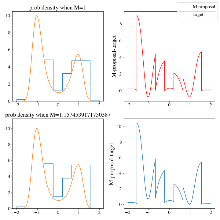
We dont expect this \(M\) to give us an estimate of the acceptance, so we’ll have to run a small trial of 500 samples first to approximate the acceptance ratio:
_ , ratio = rejection_sample(500, target_dist, hist_up, m=M)
accepted_samples, ratio = rejection_sample(int(N/ratio), target_dist, hist_up, m=M)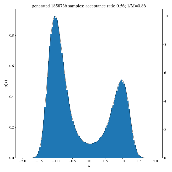
And there we go: no norm, no problem.
Optimization and Scaling
An easy optimizaton would be to edit the upper_histogram function to evaluate the midpoint as well as the ends of the intervals when calculating the height of each box. This would help improve the algorithm in stuations where the regions are not monotonic. Something like this…
counts = np.max( (target_dist(bins[:-1]),(target_dist(bins[:-1])+target_dist(bins[1:]))/2,target_dist(bins[1:])), axis=0 )Of course, you can do even more than just the midpoint, but there will be a balance in terms of how many points it is feasilbe to check. This kind of thinking gets even more important when we start thinking about higher dimensions. This brings us to the major question at hand: how does it scale into higher dimensions.
Extending the method to high dimensonal histograms should be pretty straightforward in theory:
- coarse grain the space
- for each cell in the coarse graining, evaluate the “corners” and take the height to be the max among the corners
- potentially also evaluate the center to try to account for non-monotonic regions
We can see how the evaluation of many points inside of a cell isn’t going to play that well in high dimenions because if you coarse grain an d dimenional system into n sections along each dimension you have \(n^d\) boxes, each having \(2^d\) corners. All of the sudden we are starting to evaluate a lot of points here…
This topic has turned out to be quite a bit more interesting that I originally expected. I think this deserves some more thought. Expect another installment sometime in the near future.