revenge of the "sampling from an arbitrary distribution"

note: part 3 of a series on sampling from arbitrary distrbutions, I suggest reading the second one before continuing

Refresher

Recall that our last post ended with a question about scalability and efficiency. We had built a basic framework that allowed rejection sampling, with relativelt higher acceptance rates than the uniform proposal distrbution allowed. However, we never tested if our full pipeline was acually faster than the naive uniform method. So, we will begin with this.

As a reminder, we built out some tools in the previous posts. I am not going to re-write them here, but lets recall what they are:

• target_dist : a function that returns a value from a (normalized or unnormalized) pdf when given a value or array of values. this is what we want to sample from.
• proposal_dist : an easy to sample from distribution object, it’s most important attributes are .sample(\(N\)) and .pdf(\(x\)). The sample method returns a sample of \(N\) points from the distibution and the probability density associated with them. The pdf is just the probability density evaluated at \(x\).
• HistDist : a distribution object that is initialized with a histogram (set of bins and counts), bundling it so it can be treated like a valid proposal_dist
• upper_histogram : takes in a set of bins and a target distribution to make a “smart” histogram that approximates the target distribution. In the previous post, we showed that this can perform quite a bit better than the built in np.histogram object for rejection sampling
• find_M : a function that takes in the proposal and the target distrbutions and a set of training points, \(x\). It then finds the smallest possible value for the hyperparameter \(M\) for rejection sampling.
• rejection_sample a function that takes in an integer \(n\), the proposal and the target distrbutions, and a value for M. It then performs rejection sampling using \(n\) independent samples from the proposal distributon. It outputs a list of accepted samples, which are sampled according to target_dist, as well as the ratio of accepted samples to \(n\)

Comparing the uper histogram method to the uniform distribution

So, with this in mind, lets compare our HistDist distribution object and a simple uniform distibution based on np.random.uniform. First, well need to wrap the numpy uniform distribution so we can fit it into our pipeline:

 class uniform_sampling_dist():
    def __init__(self, min, max):
        self.min = min
        self.max = max
    # it just needs these methods to play ball, so not a big deal                                                    
    def sample(self, N):
        return np.random.uniform(self.min,self.max,N), np.ones(N)/(self.max-self.min)
    def pdf(self, x):
        return np.ones(x.shape)/(self.max-self.min)

and for our target distribution we will use a bimodal distribution:

#since I am primarily motivated by physics, let's use a thermal distribution associated with a potential energy function
def target_dist(x):
    U = 2*x**4 - 4*x**2 + .3*x
    return np.exp(-U)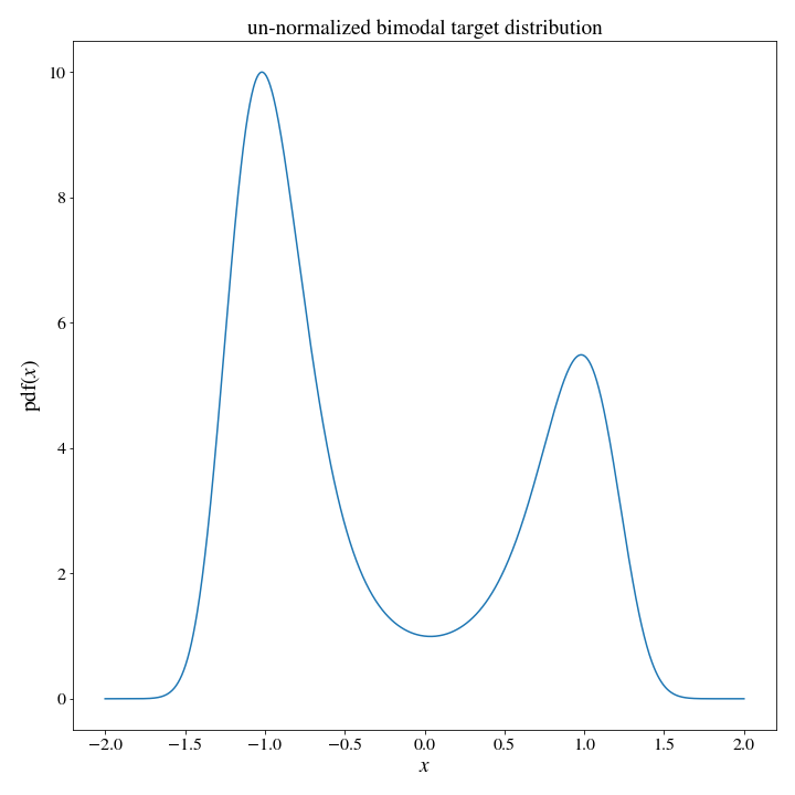

Ok, we can now set up a test for how long it takes a upper_histogram proposal, and how long it takes a uniform_sampling_distribution to pull, say, 1 million samples from this target distribution:

# we can see that the distribution is basically zero outside of [-2,2], so lets restrict our range
xmin, xmax = -2,2
# setting some parameters
training_resolution = 250
histogram_resoluton = 5
N = 1_000_000
# initialize a uniform distribution, and our smart histogam distribution
proposal_unif = uniform_sampling_dist(xmin,xmax)
bins = np.array(np.linspace(xmin, xmax, histpgram_resolution*int(xmax-xmin)))
proposal_hist = HistDist(*upper_histogram(bins, target_dist))

# find M for both proposal distributions
x=np.linspace(xmin, xmax, training_resolution*int(xmax-xmin))
M_u, _ = find_M(target_dist, proposal_unif, x, plot=False)
M_h, _ = find_M(target_dist, proposal_hist, x, plot=False)

# because we havent restricted to normalized distrbutions, we will have to figure out the acceptance ratio with a small trial run
_, ratio_h1 = rejection_sample(1000, target_dist, proposal_hist, m=M_h)
_, ratio_u1 = rejection_sample(1000, target_dist, proposal_unif, m=M_u)

Ok, now we are ready to run the speed tests, I decided to run this test in a notebook, so let’s use the ipython %%timeit magic. Here is the result:

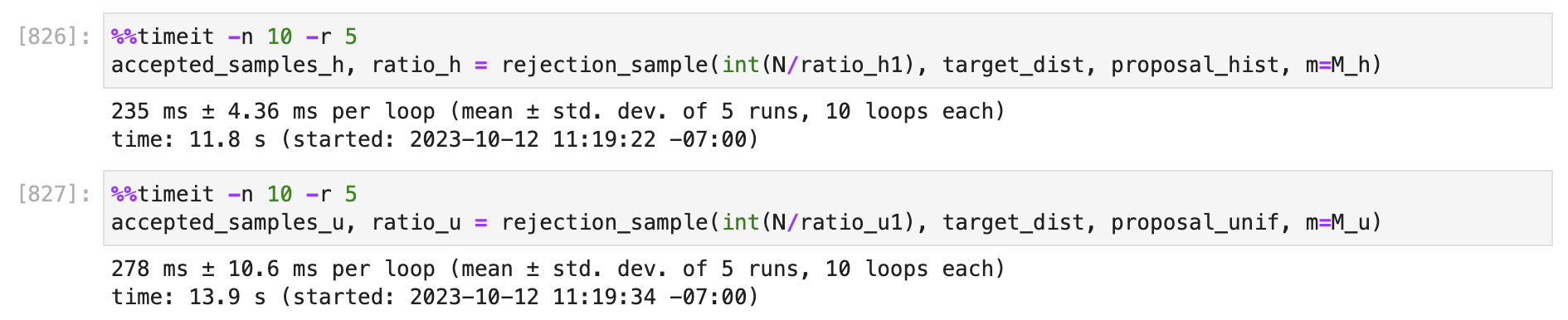
So far this doesnt look like much of an improvement for quite a bit of overhead, BUT this is a situation where uniform actually does very good. The reason is that we knew the appropriate domain to check: nealy everwhere in our uniform domain had high probability density in the target pdf. If we simulated a situation where we didnt know the domain so well we could see a better performance by the smart histogram vs the uniformk. In fact, this is actually a better model of how things behave in higher dimensions.

The curse of dimensionality

We can imagine that the pdf is composed of some number of “features” in the state space. Each feature being a region that has non-negligible probability density. For example, lets say that the target pdf above has only one feature with a length \(L\) of about 3 units (from -1.5 to 1.5). In the case above, we set the domain we look at to have a width \(V\) of 4 (from -2,2). THe probability of a uniform disribution hitting somewhere inside the high proability region associated with the deature is \(L/V = .75\). Now, lets say the feature was in 2D instead. Even if we have as good information about the second dimension (for the sake of argument lets say the feature is the same size in the second dimension), then the probability of hitting the featue in a uniform distribution is \((L/V)^2 \approx .56\), since the feature will have a size of \(L^2\)and the domain will have a size \(V^2\). Thus, as we scale up to high dimensional probability distributions, the uniform disribution will have a harder and harder time hittig the regions with high probability.

So, in order to simulate this kind of behavior, lets compare some cases where the domain of values we look at is much larger than the size of the feature. To simuate a \(n\) dimensional case, we should have the domain be \((1/.75)^n\) times larger than the feature size (4 units). Thus, simulating a 2D feature would give us a domain of (-3.5,3.5) and simulating a 6D feature (a probability distribution on a 3D phase space, for instance) gives a doman of about (-11,11).

Returning to the code above and changing xmin and xmax accodring to these values yields a speed up of 2.4X for the “2D” case, and a speedup of 4.2X for the “6D” case when comparing the smart histogram to the uniform distribution. Realistically, we are wanting to automate this process, so we can rely on setting such a nice tight window for our distribution, it would be more realistic to have our base window be a more conservative (-3,3) rather than the very tight window of (-2,2). This will also have an effect on the performance scaling, yielding a window of (-4.5,4.5) for the 2D and (-23,23) for the 6D case. WHile we can interpolate the speedup for the more conservative 2D window, after runnng another test for the conservative 6D window, I found the speed up to be 7.7X.

Thus, it does seem there is a path for scaleability here– but, as usual, it isnt as simple as we might have hoped. The speedup could probably be improved by not scaling the number of histogram bins linearly with the size of the domain (I expect this is why we start to loose efficiency for large domains). And, we havent even implemented the “smarter” histogram discussed at the end of the last installment that compares the pdf at both the corners and also the midpoint for each bin when choosing the weights. THese are pretty simple additons to what we already have, so I will eave them as an “exercise for the reader”.

Can we do better?

Well, the answer is almost certainly yes. However, wether the extra overhead of more involved methods is worth it is a different question. The method discussed above is simple and intuitive, and doesnt involve much fancy coding. The essential task is to establish a proposal distrbution that is:

• similar to the target
• quick to sample
• generated automatically
• quick to generate

And all fo these things involve tradeoffs. For example, the more time you spend building the proposal distribution– the closer it will be to the target; you tade off one time for anther. But a more complicated model is also going to be slower to sample, so there is actually another trade-off as well. A potential next step would be to try using some built in density estimators from scipy and sklearn. Can these beat the upper histogram? They are certainly more robust in the generation process… but at what cost? My first intuiton would be too use the kernel density tool: sklearn.neighbors.KernelDensity.

Well, thats all for today.

Bye